How to Get Script to Continue on Next Line When Printing Mathematica

Creating and Post-Processing Mathematica Graphics

Graphics in the Mathematica Front End is an evolving topic, so I'm collecting relevant information on a separate page. On this page the focus will be on Kernel-only operation.

Running Mathematica without the Notebook interface

Accessing the Mathematica Kernel on UNIX and Mac OS X

Mathematica is a great computational tool, and the Notebook interface makes it an almost self-contained system for doing calculations and documenting your work. However, there are some situations where one does not need or even want the interactive Notebook interface. For example, you may want to do a quick calculation while doing some work in the Terminal, or run Mathematica remotely without access to the graphical desktop.

The solution for this is to invoke an instance of the Mathematica Kernel from the command line. How you do this depends on where you are. I've been using this access method on various UNIX and Mac OS X systems at least since 1998, and it has worked with all versions of Mathematica so far.

• On a UNIX server (no longer available on the general-purpose account called "shell" at the University of Oregon, but on the research cluster hpc), you could be logged in through a text terminal session. Then if you type math, the Kernel will start up and you'll see the following:

  login> math Mathematica 7.0 for Linux x86 (64-bit) Copyright 1988-2009 Wolfram Research, Inc.  In[1]:=            

  If you don't see this, type echo $PATH and make sure that the directory path to the math command is in the list. A common path to try is /usr/local/bin/math.

• On a Mac running OS X, Mathematica is installed in the Applications folder, e.g., under the name Mathematica. Assuming this is the case on your system, you can invoke the Kernel from the command line by typing
  "/Applications/Mathematica.app/Contents/MacOS/MathKernel"
  If you're on an Intel 64-bit machine, you may have to execute MathKernel64 here (depending on your Mathematica version). In fact, you may want to follow the instructions at Wolfram's Mac support FAQ if it applies to your processor.

  Needless to say, this is one of the great advantages of working with UNIX, Linux or Mac OS X: you can in principle start as many copies of your Mathematica Kernel as your license allows, even while the "proper" Notebook Mathematica is running.

  If you do this kind of thing often, you'll want to define an alias such as

  alias math="/Applications/Mathematica.app/Contents/MacOS/MathKernel"            

  (in bash, the default shell under OS X) or

  alias math "/Applications/Mathematica.app/Contents/MacOS/MathKernel"            

  (in csh syntax). That way, the command math will work the same way on UNIX and Mac OS X machines.

  Another solution is to define a wrapper script in your PATH, e.g., /usr/local/bin/math. In this executable script, I have only two lines:

  #!/bin/sh /Applications/Mathematica.app/Contents/MacOS/MathKernel "$@"            

  The last approach is especially useful if you plan to call Mathematica from other programs that don't read your alias definitions. For example, LyX can invoke math as an external computer algebra system. It does so by parsing LaTeX and/or Mathematica code entered within LyX, converting to a Mathematica expression and eventually doing the reverse to add the output from math back into the LyX document as LaTeX. Here is an example: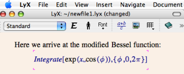

  

  With the input above, we invoke Edit > Math > Use Computer Algebra System > Mathematica and get the following: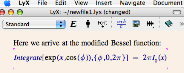

  

  The interaction between LyX and Mathematica is not perfect (in general I still prefer to have a Notebook and a LyX window open side by side, and copy/paste between them), but it illustrates the utility of the Kernel.

  To copy and paste equations between Mathematica and Lyx (or any LaTeX editor), follow the examples given on a separate page.

  There is also an interactive Mathematica mode for xemacs: mathematica-mode by Jim McCann Pivarski. This mode allows you to open an interactive Kernel session from within xemacs, with the added benefit of some useful keyboard shortcuts and (customizable) syntax highlighting. This can be quite useful when combined with JavaGraphics as described below.

  As another example for a usefull application of the, the Mathematica Kernel can even be invoked from the interactive notebook-like interface of Sage, an open-source comptetitor to Mathematica that is based on Python.

• For user-specific customizations that apply to all your Mathematica sessions, you should use the initialization file ~/Library/Mathematica/Kernel/init.m. In this file, you can place Mathematica commands such as AppendTo[$Path,"~/Documents/Mathematica"] (this example assumes that I want to automatically look for external files in ~/Documents/Mathematica).
• To create command-line scripts that accept input parameters, follow the instructions in the Mathematica (version 8) tutorial located at tutorial/MathematicaScripts in the Help browser. Note: there is a bug in MathematicaScript that doesn't allow you to pass more than three command line arguments to a script. A better way to write a script is given in the following template (see this post):

  #!/Applications/Mathematica.app/Contents/MacOS/MathKernel -script Print[$CommandLine[[3;;]]]            

Graphics output from the Kernel

Mathematica can produce graphics without invoking the (notebook) FrontEnd. One way is to export to files, as will be discussed below. But there's also a way to make graphics appear on-screen from within a Kernel-only session (note that this requires a windowing system, e.g., an X terminal):

<<JavaGraphics` Plot[{BesselJ[0,x],BesselJ[1,x]},{x,0,1},PlotStyle->{Hue[.5],Hue[1]}]        

Although this is a bit slow because it involves JLink (Java), it provides graphical feedback for your Kernel calculation without the need to open a notebook. Compared to running Mathematica through a remote X-window connection over the internet, the JavaGraphics output is really quite fast.

Running the Kernel as a batch job

The Kernel is of course much more than just a calculator replacement. Using the command-line invocation just described, you could use the Kernel to run serious computations on a remote server. However, there are two problems:

1. Making a Mathematica program file that can produce figures and other output non-interactively.
2. How to launch a Kernel job that keeps running after you log out.

The steps one needs to take are discussed next.

1. The Mathematica Kernel can be fed commands in different ways:
   • One approach is to start the Kernel as explained above, then load a text file with extention .m (e.g., foo.m by typing <<foo.m. Here, foo.m contains Mathematica commands such as Print["Hello World"].
   • Another way to tell the Kernel what to do is to specify a program file on the command line. Under UNIX, you would type

     math -run "<<input"                

     The -run option causes the command in quotation marks to be executed by the Kernel. Here, the command is to load the file named input. It does not matter whether that file has the extension .m or not, but its contents have to be Mathematica statements. We will use this below to start a batch job.

   Turning to the contents of the command file, there is the problem that we need some way of receiving output from the process. Textual output will be displayed directly in your terminal, but graphics output will create error messages if the Kernel does not know where to send the graphics. Here is an example for the file named "input" that shows how this problem is solved (the following is for Mathematica < version 6; for higher versions you shouldn't expect graphics to work without a windowing system):

   SetOptions[Plot,DisplayFunction->Identity] a=Plot[Cos[2*x],{x,0,Pi}] Export["a.eps",a] Exit[]            

   You can of course also enter these same commands interactively to see what they do. The first line has to be given only once, and it makes sure that all subsequent Plot commands produce no direct output. Instead, the output is stored in a variable a. The last line generates an Encapsulated Postscript file in you current working directory, named a.eps.

   Although the above still works with Mathematica version 6 on Mac OS X, you may have to modify the procedure slightly when logged in through a terminal session. In that case, you may get the error

   Export::nofe: A front end is not available; export of EPS      requires a front end.            

   The quick fix for this is to leave out the SetOptions line and export the expression in a as a text file: Export["a.m",a,"TEXT"]. The resulting file a.m can then be displayed in Mathematica's Front End using <<a.m, from where one can finally proceed to export other graphics formats such as EPS.

2. Having discussed the creation of command files, the last step is to make it possible to run command files over night, or longer, without having to stay logged in on the server. The first step is to modify the above to

   math -noprompt -run "<<input"            

   or alternatively

   math -noprompt -script input            

   What this does is to tell Mathematica not to show the interactive command prompt discussed earlier, but to execute silently all the commands contained in the file named "input". In the absence of a prompt, it is essential that the input file terminates the Kernel when finished. This is ensured by making the last line of the input file read Exit[] (or equivalently: Exit). Here is an example that mindlessly generates a list of twenty identical plots, just so we have time to log out before the execution finishes; save it as, e.g., test.m (the file name is arbitrary):

   Print["Hello, starting plots!"] SetOptions[DensityPlot,DisplayFunction->Identity] a=Table[DensityPlot[Sin[Sqrt[x^2 + y^2]]^2/(.001 + x^2 + y^2), {x, -13, 13}, {y, -13, 13}\ , Mesh ->  False, PlotPoints -> 300], {i, 1, 20}] Do[Export["a"<>ToString[i]<>".eps",a[[i]]],{i,1,20}] Exit[]            

   Remember, in Mathematica ≥ 6 you'll probably be best off exporting your raw data instead of trying to create graphics in a batch job (because the whole interactive paradigm of versions ≥6 causes graphics to be overwhelmingly handled by the Notebook instead of the Kernel).
3. Submitting your batch job: this depends on the system you're logged in to.

   If you're running the job remotely on your own Mac, then to launch this program in a way that does not get killed when you log out, type the following:
   nohup nice math -noprompt -run "<<test.m" > output &
   The & at the end is important, and the file named output catches any text output that your job might generate.

   On the other hand, if you're working on a cluster such as hpc, follow the procedure outlined in the cluster documentation: usually it involves simply launching your script with the qsub command.

Remote Mathematica Notebook Sessions

If you need graphical features specific to version 6 or above, there is no way around a notebook interface. Over a remote connection, this will of course require a lot of bandwidth. My recommendation here would be to avoid a remote X-window connection and use vnc (screen sharing) instead, if the server supports it. The network traffic for a vnc connection is smoother and much more responsive than for a remote X connection with Mathematica's highly interactive notebook features.

To access Mathematica in all its graphical interface glory on a remote Unix/Linux server such as the UO hpc, the main issue that can trip you up is a lack of installed fonts. Ideally, all you have to do (on a Mac) is: ssh -Y hpc.uoregon.edu, followed by mathematica at the command prompt.

In all likelyhood, this won't work when you try it for the first time. So here are the steps to fix things:

• If things freeze up, go to the terminal, press Ctrl-z and type kill -9 %1 (if necessary, replace %1 by the appropriate number output by jobs).
• Log out (exit), go to your local home directory in the Terminal (cd) and type scp -r hpc.uoregon.edu:/usr/local/mathematica7/SystemFiles/Fonts . followed by mv Fonts .fonts (replace mathematica7 by whatever version you wish to run). This copies the fonts from the remote server to your own computer.
• Type cd .fonts and then mkfontdir BDF Type1.
• Now go back by typing cd, create a new folder with mkdir .xinitrc.d (if it doesn't already exist) and then type this as a single line: printf "xset fp+ $HOME/.fonts/BDF\nxset fp+ $HOME/.fonts/Type1\nxset fp rehash\n" >> ~/.xinitrc.d/setFontPaths.sh
• Make this file executable by typing chmod 755 ~/.xinitrc.d/setFontPaths.sh.
• Restart your X server and go back to the first paragraph. Now if you launch mathematica on hpc, the notebook should start up.

At this point you'll see what I meant when I recommended vnc over X.

---

noeckel@uoregon.edu

Last modified: Tue May 8 13:30:15 PDT 2012

downthaverse.blogspot.com

Source: https://pages.uoregon.edu/noeckel/Mathematica.html

Share this post